YAYYYY TRANSFORMATION MATRICESSS YIPPPEEEEE
Combining Maps of Sections
Before we can combine the maps of the different sections, we need to determine the transformation matrices between the different scans.
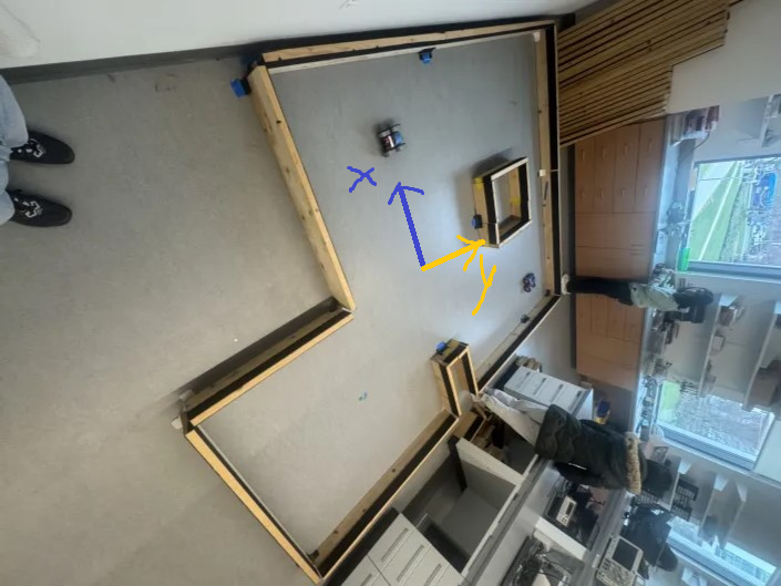
We first need to define the coordinate system of the robot and the world. We define the robot's coordinate system as having the x-axis pointing forward, the y-axis pointing to the left, as this is what the IMU
uses so it's easy as shown below.
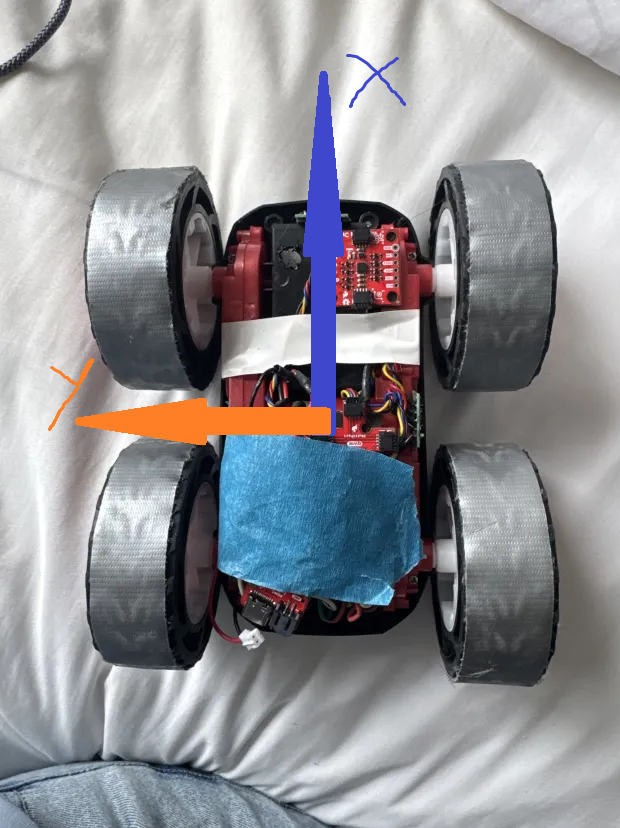 The world axes are defined by the coordinates that are already placed.
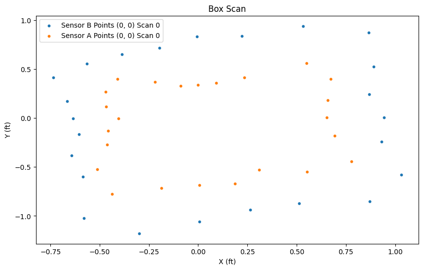
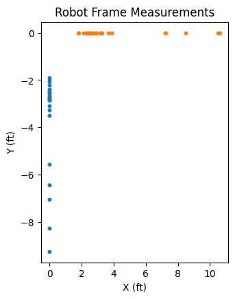
From the robot's frame, the distance measurements look like this, where sensor A is on the side of the robot and sensor B in in front. The robot's sensors are always rotating with the robot
so it just looks like two straight lines of distance measurements. Each point on the plot is in the form:
\[
\begin{bmatrix}
B_{dist} \\
0
\end{bmatrix}
\quad
\begin{bmatrix}
0 \\
-A_{dist}
\end{bmatrix}
\]
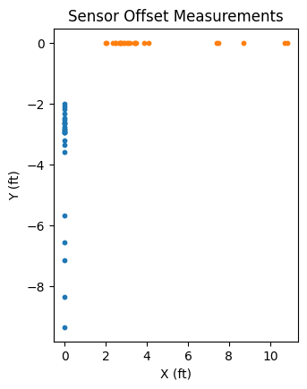
 Because the sensors are offset from the center of the robot, the distances need to be translated slightly to account for the decreased measured distance which is represented by these matrices. In this case, da was 0.109ft and db was 0.208ft.
\[
T_A =
\begin{bmatrix}
1 & 0 & 0 \\
0 & 1 & -d_A \\
0 & 0 & 1
\end{bmatrix}
\quad
T_B =
\begin{bmatrix}
1 & 0 & -d_B \\
0 & 1 & 0 \\
0 & 0 & 1
\end{bmatrix}
\]
Because the sensors are offset from the center of the robot, the distances need to be translated slightly to account for the decreased measured distance which is represented by these matrices. In this case, da was 0.109ft and db was 0.208ft.
\[
T_A =
\begin{bmatrix}
1 & 0 & 0 \\
0 & 1 & -d_A \\
0 & 0 & 1
\end{bmatrix}
\quad
T_B =
\begin{bmatrix}
1 & 0 & -d_B \\
0 & 1 & 0 \\
0 & 0 & 1
\end{bmatrix}
\]
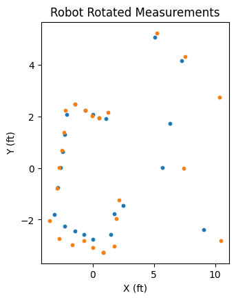
 We can then use a standard rotation matrix to rotate the points relative to the robot's rotation when it took the measurement.
\[
R(\theta) =
\begin{bmatrix}
\cos(\theta) & -\sin(\theta) \\
\sin(\theta) & \cos(\theta)
\end{bmatrix}
\]
We can then use a standard rotation matrix to rotate the points relative to the robot's rotation when it took the measurement.
\[
R(\theta) =
\begin{bmatrix}
\cos(\theta) & -\sin(\theta) \\
\sin(\theta) & \cos(\theta)
\end{bmatrix}
\]
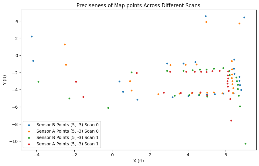
 However, we want the rotation relative to the world axis coordinates since the robot's axes weren't aligned with them on bootup. This can be found by taking a known straight piece of the
map, take the left side of that plot, and then finding the angle of it.
However, we want the rotation relative to the world axis coordinates since the robot's axes weren't aligned with them on bootup. This can be found by taking a known straight piece of the
map, take the left side of that plot, and then finding the angle of it.
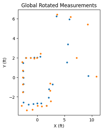
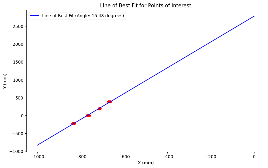 We can then rotate the points by the angle of this line to get the points in the world frame (in the matrix this is just subtracting the angle from theta).
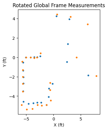
 Finally, we can then translate the points to the correct location in the world frame by using the known location of the robot when it took the measurements.
 The code for the matrix math is shown below:
sensor_to_robot_transform_B = np.array([[1, 0, 0.208333],  # translate by sensor offset
                                        [0, 1, 0],
                                        [0, 0, 1]])

sensor_to_robot_transform_A = np.array([[1, 0, 0],  # translate by sensor offset
                                        [0, 1, -0.109375],
                                        [0, 0, 1]])

def rotation_matrix(angle_yaw):
    angle = -angle_yaw - angle_rad # adding angle of robot and global frame correction
    return np.array([[np.cos(angle), -np.sin(angle), 0],
                     [np.sin(angle), np.cos(angle), 0],
                     [0, 0, 1]])

def translation_matrix(offset):
    return np.array([[1, 0, offset[0]],
                     [0, 1, offset[1]],
                     [0, 0, 1]])

# combined transformation from sensor coordinates to world coordinates
def sensor_to_world_transform(sensor, angle_yaw, offset):
    if sensor == 'A':
        sensor_to_robot = sensor_to_robot_transform_A
    elif sensor == 'B':
        sensor_to_robot = sensor_to_robot_transform_B

    robot_rotation = rotation_matrix(angle_yaw)
    robot_translation = translation_matrix(offset)

    # combined transformation
    return robot_translation @ robot_rotation @ sensor_to_robot
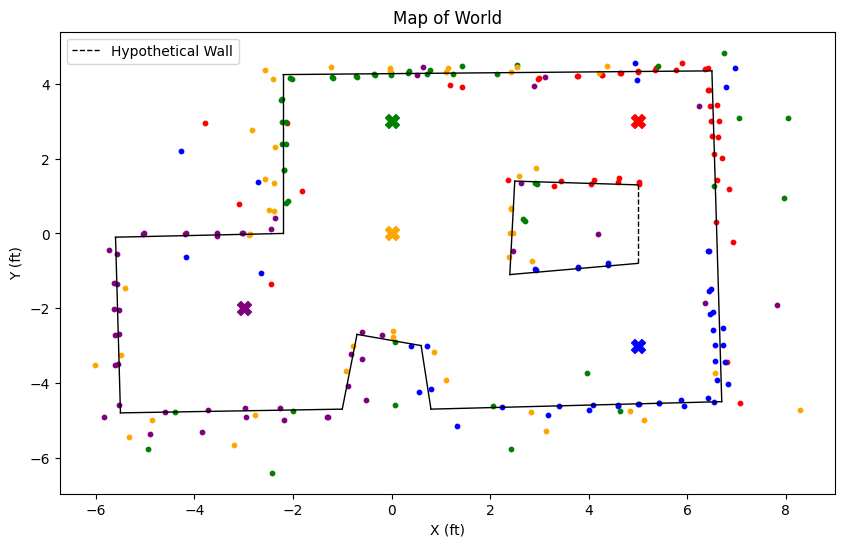
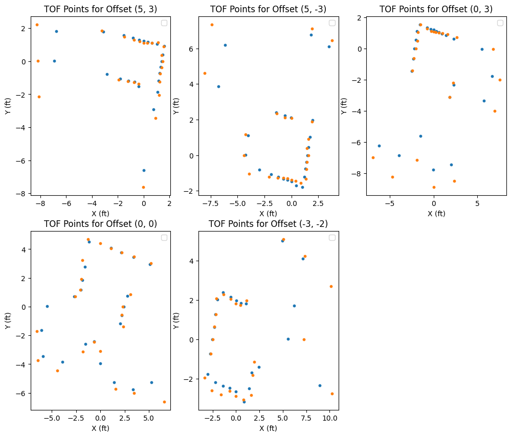
Doing this process with all the scans yields this map:
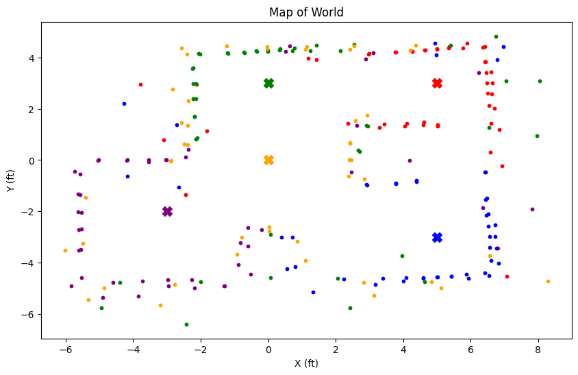 We can then estimate walls onto this plot to create a map of the world. There is a missing wall shown by the dotted line since the robot's positions of scans couldn't reach that wall to take measurements of it.