Fast Robots Lab 6

Fast Robots: Lab 7

Arduino IDE • Bluetooth • Jupyter Notebooks • PID

• Kalman Filter

Kalman Filter

This lab is about implementing a Kalman filter for state estimation of the robot's position and velocity to improve control performance.

The Weeds of It

Kalman Filter Mathematics

The Kalman filter is a way to combine information from two different sources to get a better estimate of the state of a system. In our case, we combine the data from a model of the robot's motion (the "prediction") with measurements from sensors (the "update") to get a more accurate estimate of the robot's position and velocity.

Function: $\text{KalmanFilter}(\mu(t-1), \Sigma(t-1), u(t), z(t))$

Prediction Step: \[\mu_p(t) = A\mu(t-1) + Bu(t)\] \[\Sigma_p(t) = A\Sigma(t-1)A^T + \Sigma_u\]
Update Step:

$K_{KF} = \Sigma_p(t)C^T(C\Sigma_p(t)C^T + \Sigma_z)^{-1}$
$\mu(t) = \mu_p(t) + K_{KF}(z(t) - C\mu_p(t))$
$\Sigma(t) = (I - K_{KF}C)\Sigma_p(t)$

Return: $\mu(t)$ and $\Sigma(t)$

In plain terms, we need the initial state estimate $\mu(t-1)$ and its uncertainty $\Sigma(t-1)$, the control input $u(t)$ that we applied to the robot, and the measurement $z(t)$ we got from our sensors. The robot uses $A$ to predict how the state changes without control input, and $B$ to predict how the control input affects the state and $C$ to relate the predicted state to the measurements. $\Sigma_u$ and $\Sigma_z$ represent the uncertainty in our model and measurements, respectively.

Prediction Matrices

Estimating Drag and Momentum

We have to calculate the matrices $A$, $B$, and $C$ for our system. Our equation of motion for the car is: $$\ddot{x} = \frac{u}{m} - \frac{d}{m}\dot{x}$$ where, at constant speed, $$d = \frac{u}{\dot{x}}$$ and $$m = \frac{-dt_{0.9}}{\ln(1 - 0.9)}$$ where $t_{0.9}$ is the time it takes for the car to reach 90% of its final velocity after a step input. In this case, since our state is $\begin{bmatrix} x \\ \dot{x} \end{bmatrix}$, we can derive the matrices as follows: \[A = \begin{bmatrix} 1 & 1 \\ 0 & 1 - \frac{d}{m} \end{bmatrix}\] \[B = \begin{bmatrix} 0 \\ \frac{1}{m} \end{bmatrix}\] \[C = \begin{bmatrix} 1 & 0 \end{bmatrix}\] C is 1 and 0 because we are only measuring the position $x$ and not the velocity $\dot{x}$.

We can get the values of $d$ and $m$ by performing a step response test on the robot, where we apply a step input and measure the velocity response over time.

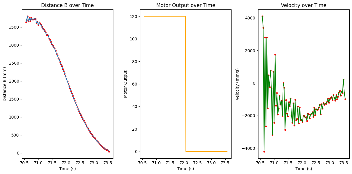
We can then fit an exponential curve to the velocity response to extract the time constant $t_{0.9}$ and constant velocity for the given PWM input of 120 and calculate $m$ and $d$. The velocity data was very noisy at the beginning due to the robot oscillating as it starts to move, causing the ToF data to be unreliable. To get around this, I only fit the curve after the first 10 points and until the input control was 0.

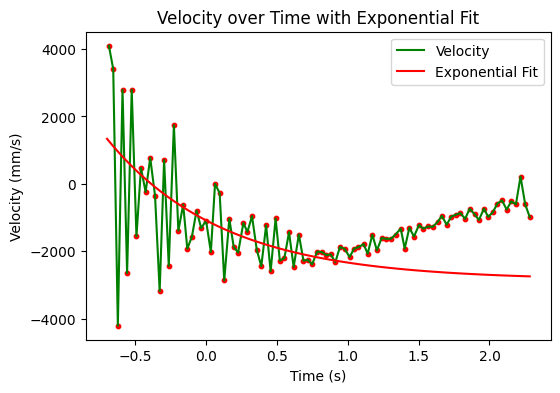
The equation of the fitted curve is: $$v(t) = 2168.301(1 - e^{-t/0.413})$$ Therefore, the steady sate velocity is 2168.301 mm/s, and $t_{0.9}$ is empiracally found to be 0.131 seconds, and we can calculate $m$ and $d$ as follows: \[m = \frac{-dt_{0.9}}{\ln(1 - 0.9)} = 0.262 * 10^{-5} \text{ kg}\] \[d = \frac{u}{\dot{x}} = 4.61 * 10^{-4} \text{ kg/s}\] So the matrices are: \[A = \begin{bmatrix} 0 & 1 \\ 0 & -17.600 \end{bmatrix}\] \[B = \begin{bmatrix} 0 \\ 38163.7 \end{bmatrix}\]

Since we are working with discrete time steps, we can also convert the continuous-time system to a discrete-time system using the following formulas: \[A_d = A*dt\] \[B_d = B*dt\] where $dt$ is the time step of our control loop, which is 0.000897 seconds. Therefore, the discrete-time matrices are: \[A_d = \begin{bmatrix} 1 & 0.000897 \\ 0 & 0.9842 \end{bmatrix}\] \[B_d = \begin{bmatrix} 0 \\ 34.265 \end{bmatrix}\]

ARHJGAGHEHRGAHGR

Noise

Since we are modelling gaussians, we need to calculate the covariance matrices $\Sigma_u$ and $\Sigma_z$ for our system. $\Sigma_u$ represents the uncertainty in the state, while $\Sigma_z$ represents the uncertainty in our measurements. $\Sigma_u$ is as follows: \[\Sigma_u = \begin{bmatrix} \sigma_x^2 & 0 \\ 0 & \sigma_{\dot{x}}^2 \end{bmatrix}\] and $\Sigma_z$ is as follows: \[\Sigma_z = \begin{bmatrix} \sigma_z^2 \end{bmatrix}\] We calculate $\sigma_x$ and $\sigma_{\dot{x}}$ via: $$\sqrt{10^2 \cdot \frac{1}{dt}} = 333.73$$ And we assume $\sigma_z$ to be 20 mm, which is a reasonable estimate for the noise in our ToF sensor measurements according to the datasheet (page 16)

This Works Right?

Python Simulation

To test that our Kalman filter implementation is correct, we can simulate the system in Python and see if the state estimates align with the data we collected from the robot in lab 5. Using the code below, we can simulate the system and plot the results. Our initial state is $\mu(0) = \begin{bmatrix} dist_0 \\ 0 \end{bmatrix}$ and $\Sigma(0) = \begin{bmatrix} \sigma_x^2 & 0 \\ 0 & 1 \end{bmatrix}$. We use the measurement noise for the standard deviation of the position, and a small value for velocity since we are fairly certain that the robot starts at rest.

def kalman_filter_step(x_prev, P_prev, u, z):
# Prediction Step
x_pred = A_d @ x_prev + B_d.flatten() * u  
P_pred = A_d @ P_prev @ A_d.T + Sigma_u 

# Measurement Update Step
y = z - C @ x_pred  
S = C @ P_pred @ C.T + Sigma_z  
K = P_pred @ C.T @ np.linalg.inv(S)  # Kalman Gain

x_updated = x_pred + K.flatten() * y 
P_updated = (np.eye(len(P_prev)) - K @ C) @ P_pred 
return x_updated, P_updated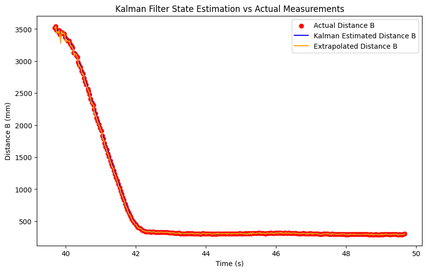

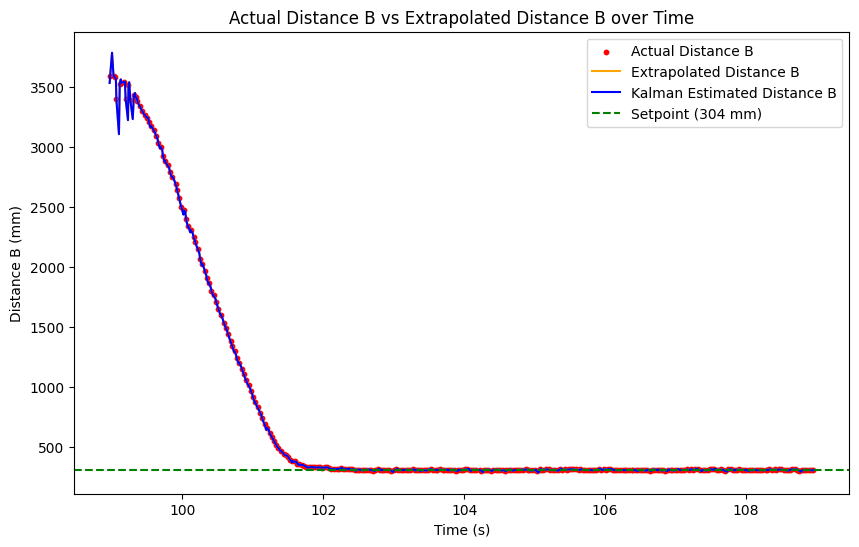
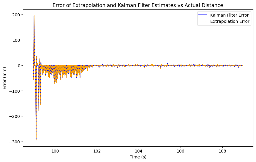
The linearly extrapolated position already closely matches the data, which makes sense because we are looping at a very high frequency and get a measurement back about once every 3 loops. The kalman filter similarly very closely matches the data as well though, indicating that our implementation is correct and our parameters are sufficiently accurate to model the system well.

For a bit of experimentation, I also tried increasing the measurement noise to 100000 mm, and as expected, the Kalman filter solely relies more on the prediction and not on the measurements, resulting in an estimate that is wildly incorrect.

Kalman Filter Simulation with Noisy Measurements

Easy Stuff Light Work

Implementing On the Robot

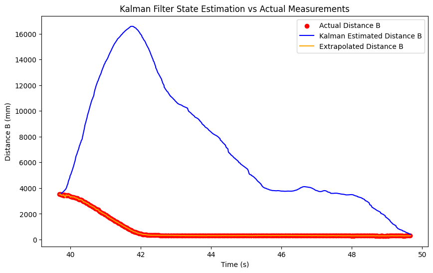
Now that we know it works, we can implement it on the Artemis. Using the same code structure, just in C without the matrix operations, we can implement the Kalman filter on the robot and see how it performs.

float step(float u, float z)
{
    // --- PREDICTION STEP ---
    // x_pred = Ad * x_est + Bd * u
    float x_pred[2];
    x_pred[0] = Ad[0][0] * x_est[0] + Ad[0][1] * x_est[1] + Bd[0] * u;
    x_pred[1] = Ad[1][0] * x_est[0] + Ad[1][1] * x_est[1] + Bd[1] * u;

    // P_pred = Ad * P_est * Ad^T + Sigma_u
    float P_p[2][2];
    float m1[2][2];
    m1[0][0] = Ad[0][0] * P_est[0][0] + Ad[0][1] * P_est[1][0];
    m1[0][1] = Ad[0][0] * P_est[0][1] + Ad[0][1] * P_est[1][1];
    m1[1][0] = Ad[1][0] * P_est[0][0] + Ad[1][1] * P_est[1][0];
    m1[1][1] = Ad[1][0] * P_est[0][1] + Ad[1][1] * P_est[1][1];

    P_p[0][0] = m1[0][0] * Ad[0][0] + m1[0][1] * Ad[0][1] + Sigma_u[0][0];
    P_p[0][1] = m1[0][0] * Ad[1][0] + m1[0][1] * Ad[1][1] + Sigma_u[0][1];
    P_p[1][0] = m1[1][0] * Ad[0][0] + m1[1][1] * Ad[0][1] + Sigma_u[1][0];
    P_p[1][1] = m1[1][0] * Ad[1][0] + m1[1][1] * Ad[1][1] + Sigma_u[1][1];

    // --- 2. UPDATE STEP ---
    if (z != -1) // Only update if sensor data is valid
    {
        // y = z - C * x_pred 
        float y = z - (C[0] * x_pred[0] + C[1] * x_pred[1]);

        // S = C * P_pred * C^T + Sigma_z
        // Since C is [1, 0], this simplifies greatly:
        float S = P_p[0][0] + Sigma_z;

        // K = P_pred * C^T * inv(S)
        float K[2];
        K[0] = P_p[0][0] / S;
        K[1] = P_p[1][0] / S;

        // x_est = x_pred + K * y
        x_est[0] = x_pred[0] + K[0] * y;
        x_est[1] = x_pred[1] + K[1] * y;

        // P_est = (I - K*C) * P_pred
        P_est[0][0] = (1.0 - K[0]) * P_p[0][0];
        P_est[0][1] = (1.0 - K[0]) * P_p[0][1];
        P_est[1][0] = -K[1] * P_p[0][0] + P_p[1][0];
        P_est[1][1] = -K[1] * P_p[0][1] + P_p[1][1];
    }
    else
    {
        // No measurement: Update estimate with prediction
        x_est[0] = x_pred[0];
        x_est[1] = x_pred[1];
        P_est[0][0] = P_p[0][0];
        P_est[0][1] = P_p[0][1];
        P_est[1][0] = P_p[1][0];
        P_est[1][1] = P_p[1][1];
    }

    return x_est[0]; // Return the filtered position
}

We drove it into a wall using the PID loop, but using the Kalman Filter to predict the position instead of linearly extrapolating the position, and the results were decent. The Kalman filter was able to accurately predict the position of the robot, except for the start where the measurements were very noisy, and the velocity estimates were similarly very innacurate. The plots are shown below:

The speed of our loop is fairly constant whether we use the extrapolated data or the Kalman filter, since in both cases, we are constantly looping at about once every 0.0089 seconds. However, compared to using the raw data, these methods greatly speed up our PID loop since we only get a new measurement to act upon every 0.0327 seconds. A video of the robot driving into the wall using the Kalman Filter distance with the PID loop is shown below:

I used Lucca Correial's website as a reference for the math and website formatting. I also used Aidan McNay's website for reference on the plotting and Python simulation. I also used Gemini to help write the code for the Kalman filter step in C and Python, as well as formatting the math in this page.