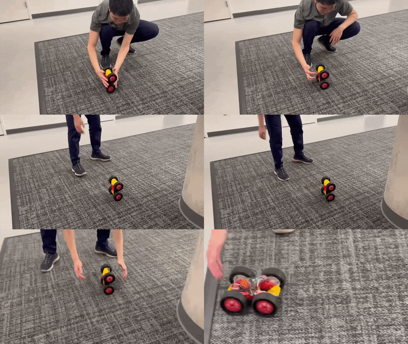
This lab is about balancing our car upright on two of its wheels, similar to a wheelie.
We will attempt to use a Kalman filter to speed up the control loop (but it performs worse than DMP),
and begin our control schema by using an LQR controller, followed by MANY iterations of tweaking the controller.
We also attemped to use a simple PID controller, but it was less effective than the LQR-based controller.
Let's do a ton of math and physics!!!!!!
System Dynamics
Before we can design our controller, we should have a model of the system dynamics.
We are modelling our robot as an inverted pendulum on a cart, with the rear axle as the pivot.
The "cart" is the wheels — mass \(M_w\), including the reflected driveline inertia.
The "pendulum" is everything that pivots about the axle: chassis, battery, Artemis, IMU. We give it mass
\(m_b\), its center of mass sits a distance \(L\) above the axle when upright, and its moment of
inertia about its own COM is \(I_{b,\text{com}}\). The parallel-axis shift gives the inertia about
the pivot: \(\alpha = I_{b,\text{pivot}} = I_{b,\text{com}} + m_b L^2\).
Inverted-pendulum-on-cart model. The pendulum is shown tilted at \(\theta > 0\) for clarity;
balance is \(\theta = 0\) (body straight up). Positive \(u\) pushes the wheel contact in \(+x\).
Coordinates. \(x\) is the horizontal position of the rear-axle contact point in the world,
and \(\theta\) is the body's pitch from vertical (positive in the \(+x\) direction). The control input \(u\)
is the net horizontal force applied at the wheel contact.
Assumptions. Motor commands map directly to \(\dot x\) of the cart.
The wheels' own rotational inertia is folded into \(M_w\), so we don't need a separate wheel state.
(We also ignore wheel friction and any out-of-plane motion. The PWM-to-Newtons
calibration is a separate hardware constant, not part of the dynamics.)
Kinematics
The cart sits at \((x, 0)\). The body's COM, offset by the pendulum at angle \(\theta\), is at:
KE has three contributions: cart translation, body COM translation, and body rotation about its own COM.
With total mass \(M = M_w + m_b\):
\[ T = \tfrac12 M_w \dot x^2 + \tfrac12 m_b\, v_{\text{COM}}^2 + \tfrac12 I_{b,\text{com}} \dot\theta^2
= \tfrac12 M \dot x^2 \,+\, m_b L \cos\theta \cdot \dot x \dot\theta \,+\, \tfrac12 \alpha \dot\theta^2 \]
Only the body's height varies with the coordinates, so:
\[ V = m_b g L \cos\theta \]
\(V\) is maximum at \(\theta = 0\), which is exactly what makes the upright position an
unstable equilibrium.
Euler-Lagrange Equations
The Lagrangian is \(\mathcal L = T - V\). The generalized forces are \(Q_x = u\)
(the motor force enters through the wheel contact, doing work along \(x\)) and \(Q_\theta = 0\).
Working out \(\frac{d}{dt}(\partial \mathcal L / \partial \dot q) - \partial \mathcal L / \partial q = Q_q\)
for each coordinate:
For \(x\):
\[ M \ddot x + m_b L \cos\theta \cdot \ddot\theta - m_b L \sin\theta \cdot \dot\theta^2 = u \]
For \(\theta\) (the cross \(-m_b L \sin\theta \cdot \dot x \dot\theta\) terms from the time derivative and \(\partial \mathcal L/\partial \theta\) cancel):
\[ m_b L \cos\theta \cdot \ddot x + \alpha \ddot\theta - m_b g L \sin\theta = 0 \]
Small-Angle Linearization
Balance operates near \(\theta = 0\), so we substitute \(\sin\theta \approx \theta\),
\(\cos\theta \approx 1\), and drop \(\dot\theta^2\) (second-order small). Defining \(\beta = m_b L\),
the linearized system becomes:
\[
\begin{bmatrix} M & \beta \\ \beta & \alpha \end{bmatrix}
\begin{bmatrix} \ddot x \\ \ddot\theta \end{bmatrix}
=
\begin{bmatrix} u \\ m_b g L\,\theta \end{bmatrix}
\]
The mass matrix is symmetric (a property baked into the Lagrangian structure) with positive
determinant \(\det = M\alpha - \beta^2\). Inverting and solving:
\[ \ddot x = \frac{\alpha}{\det}\,u \;-\; \frac{\beta\, m_b g L}{\det}\,\theta \]
\[ \ddot \theta = -\frac{\beta}{\det}\,u \;+\; \frac{M m_b g L}{\det}\,\theta \]
The negative off-diagonal signs are the momentum-conservation effects from the sanity check:
push the cart forward, body tilts back; lean the body forward, cart drifts back.
State-Space Form
With state \(\vec x_4 = [\,x,\ \dot x,\ \theta,\ \dot\theta\,]^T\):
The eigenvalues of \(A_4\) are two zeros (the integrators for \(x\) and \(\theta\)) and a real
pair \(\pm\sqrt{M m_b g L/\det}\). The positive root is the unstable fall mode; its
reciprocal is the fall time constant — about 70 ms for our robot's parameters, which means the
balance loop shoud ideally run at least 5× faster, but we'll attempt and give up on speeding it up.
Dropping the Position State
Our robot has no wheel encoders, so absolute position \(x\) is unobservable. Penalizing it in
\(Q\) wouldn't make the controller actually know \(x\), so we drop it and use the 3-state
\(\vec x_3 = [\,\dot x,\ \theta,\ \dot\theta\,]^T\):
\[
A = \begin{bmatrix}
0 & -\dfrac{\beta\, m_b g L}{\det} & 0 \\
0 & 0 & 1 \\
0 & \dfrac{M\, m_b g L}{\det} & 0
\end{bmatrix},
\quad
B = \begin{bmatrix} \alpha/\det \\ 0 \\ -\beta/\det \end{bmatrix}
\]
This is the model the design notebook hands to scipy.linalg.solve_continuous_are to
get the LQR gain \(K\). The notebook then divides \(K\) by the force-to-PWM calibration \(k_f\)
and converts \(\theta\), \(\dot\theta\) from radians to degrees so the Artemis can apply
\(u_{\text{PWM}} = -K \cdot \vec x_3\) using the IMU's native units directly.
We tried....
Kalman Filter for IMU Readings
The fall time constant for our robot is about 70 ms, which means that ideally we would want our control loop to run at least 5× faster than that to have good stability margins.
However, when we use the DMP on the IMU, we can only get readings at about 50 Hz, which is not fast enough to get a 5x speed.
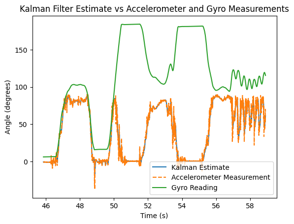
We attempted to use a Kalman filter to fuse the DMP readings with the raw accelerometer and gyroscope readings from the IMU, which are available at a much higher rate (about 200 Hz), to get faster state estimates for our controller.
The code for the Kalman filter is the same as the one used in Lab 7, just changing the state transition and measurement matrices to fit our new state space model.
We want to model the angle as $$\hat{\theta}_{new} = \hat{\theta} + (\omega - b) \Delta t$$
where $\hat{\theta}$ is the previous angle estimate, $\omega$ is the gyroscope reading, $b$ is the gyro bias, and $\Delta t$ is the time step.
The state matrices are as follows:
\[
A = \begin{bmatrix}
1 & -\Delta t \\
0 & 1
\end{bmatrix},
\quad
B = \begin{bmatrix} \Delta t \\ 0 \end{bmatrix},
\quad
C = \begin{bmatrix} 1 \\ 0 \end{bmatrix}
\]
And the process and measurement noise covariances are as follows:
\[
Q = \begin{bmatrix}
\sigma_{\dot{\theta}}^2 & 0 \\
0 & \sigma_{bias}^2
\end{bmatrix},
\quad
R = \begin{bmatrix} \sigma_{\text{acc}}^2 \end{bmatrix}
\]
We measured that the dt between the raw IMU readings is about 4 ms, which we used as our time step for the Kalman filter and is way faster than the ~17ms of the DMP.
We landed on \(\sigma_{\dot{\theta}} = 0.001\), \(\sigma_{bias} = 0.000001\), and \(\sigma_{\text{acc}} = 0.01\), which makes sense since the gyroscope readings are pretty accurate and we don't expect the bias to change much, while the accelerometer readings are pretty noisy when the robot is moving around.
This worked pretty well while moving the robot by hand as shown below:
However, when we actually tried to use the Kalman filter estimates in our control loop, the performance was much worse than just using the DMP readings directly, which was surprising since the Kalman filter estimates were much faster than the raw DMP readings.
We think this is because the Kalman filter was still more noisy than the DMP, with a single wrong reading making the robot stop rotating or shoot off immediately.
We attempted to tune the noise covariances to try to get faster estimates from the Kalman filter, but we couldn't get it to perform better than just using the DMP readings directly, so we ended up using the DMP readings for our controller instead of the Kalman filter estimates.
Getting Gains and Immediately Disregarding Them
LQR Controller
We used the state-space model derived in the previous section to design an LQR controller for our robot to get the optimal gain matrix \(K\) for our system.
The Q matrix was:
$$
Q = \begin{bmatrix}
1.0 & 0 & 0 \\
0 & 200.0 & 0 \\
0 & 0 & 10.0
\end{bmatrix}
$$
Since we want to penalize deviations from the upright position more than our angular velocity and much more than deviations from the desired velocity.
And the R matrix was a scalar with value 1.0, which means we are penalizing the control effort equally across all states and inputs.
We then implemented the control law \(u = -K \cdot \vec x\) on the Artemis, where \(\vec x\) is the state vector consisting of the angle and angular velocity of the robot.
This expands to \(u = -K_1 \dot x - K_2 \theta - K_3 \dot\theta\), where \(K_1\), \(K_2\), and \(K_3\) are the elements of the gain matrix \(K\).
The code for this is shown below which returns a PWM value to command our motors. We want to have 0 angular and forwards velocity since we want to get to a stationary upright position.
int compute(float theta_deg, float theta_dot_deg_per_s, int last_pwm)
{
    // lowpass pwm for velocity cause it'll be relative to the avg pwm
    float pwm_as_mps = pwm_to_mps * (float)last_pwm;
    xdot_est = xdot_alpha * pwm_as_mps + (1.0f - xdot_alpha) * xdot_est;

    float theta_err     = wrap_diff_deg(theta_deg, theta_balance_deg); // making sure we're [-180,180]
    float theta_dot_err = theta_dot_deg_per_s;
    float xdot_err      = xdot_est;

    // stop running if we've fallen
    if (fabs(theta_err) > tipover_threshold_deg) {
        tipped_over = true;
        return 0;
    }

    // u = -K * x_err
    float u = -(K_xdot * xdot_err + K_theta * theta_err + K_thetadot * theta_dot_err);

    // deadband
    if (fabs(u) < pwm_zero_band) {
        return 0;
    }
    if (fabs(u) < (float)pwm_min) {
        u = (u > 0) ? (float)pwm_min : -(float)pwm_min;
    }
    if (u >  (float)pwm_max) u =  (float)pwm_max;
    if (u < -(float)pwm_max) u = -(float)pwm_max;

    return (int)u;
}
However, we found that the performance of the controller with the initial gain matrix was pretty bad, with the robot oscillating a lot and not being able to balance for more than a second if at all.
Instead of trying to tune the Q and R matrices to get a better gain matrix, we decided to just manually tune the gain matrix by hand.
Below is a grid of (the best intermediate) videos of us tuning (had to cutout about an hour of straight fails).
GODDAMMIT SAKJFNKAGSNDAKSFJNG AGAIN????!?!?
RIP PUYO PUYO
So....as an aside from the technical portion of this report....during the beginning of my testing, I was tuning the gains when suddenly, my car stops moving.
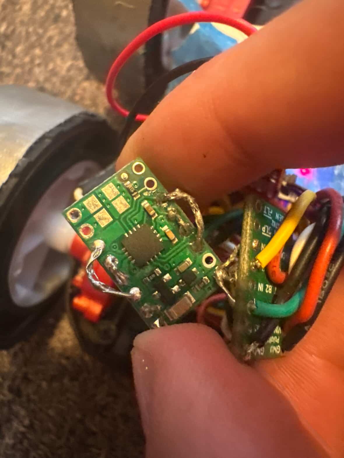
And then when I test it by going forwards, it starts smoking :D. I never checked the soldering on Puyo Puyo that closely after Puyo's death (in Lab 8).
It turns out the motor drivers are soldered like so, and are cramped together in the tiny divot in the car.
Somehow this wasn't a problem until the final lab, but the two exposed metals on the motor drivers touched and started to smoke, and cooked the car.
So thank you Ananya for letting me borrow your car for the rest of the lab, and thank you Puyo Puyo for being a good friend and a good car for the past 4 labs. RIP Puyo Puyo :(
Here is a video of it dancing before it died, having the "time of it's life." (listen to the music for full effect)
*spits on it* shouldn't have even tried
PID Controller Attempt
After struggling to get the LQR controller to work well, I attempted to implement a PID controller instead, since it is a much simpler controller and I thought it would be easier to tune.
It is a simple PID controller using the angle error from the DMP readings, with the same deadband and tipover threshold as the LQR controller.
However, I found that the performance of the PID controller was even worse than the LQR, with the robot not being able to balance at all.
We tried tuning it for a while, but we couldn't get it to work well, so we ended up just using the LQR controller for the rest of the lab.
Below is a video of the PID controller in action, which is pretty bad, but it was fun to try out and see how it performs compared to LQR.
YAYAYYAY
It Kinda Works?!?
After tuning the LQR controller for a while, we found that it works best when the gain for theta is about 60x larger than the gain for theta dot, and the gain for x dot should be 0 because who cares how fast we're going forwards or backwards as long as we don't fall over.
The specific gains we ended up with were \(K = [0.0, 41.6678, 0.6928]\).
Below is a video of the robot balancing with these gains.
In this trial, the gains looked fine, but it looks like it was trying to stablize a bit off from the upright position, which is why it was oscillating around that point instead of the upright position.
Instead we changed the setpoint angle slightly and tried again as shown below, which worked pretty well!
We also wanted to see how it would do on different surfaces, so we tried it on wood, which is much more slippery than the carpet. It performed worse as expected
since the wheels have less grip.
Stretch Goals
Making It Flip Up (or trying)
We wanted to see if we could get the robot to flip up from rest, which is a much harder problem than just balancing, since it requires the robot to swing up and gain enough energy to reach the upright position, but not move so fast that it shoots off the other way.
We attempted to have it drive forwards and backwards at just the right timing to get it just barely to swing up since our current implementation of the LQR controller already automatically waits to start trying to balance until it detects that the robot is close enough to the upright position.
However, we couldn't get it to work well, since it would move too fast and shoot off the other way, or it would move too slow and not gain enough energy to swing up. Additionally, our current tuning
of the controller is pretty finicky - we have to start in almost an exact upright position to balance right. Below are a couple attempts though.
While trying to get it to flip, we added weights to the robot to make it easier to swing up. While this didn't end successfully, it led us to discover that the robot balances much better with the weights on.
This makes sense since a higher center of mass means the robot has more inertia and is less affected by small disturbances, which makes it easier to balance.
WAIT OMG IT WORKS SO WELL
Final Results
Adding the weights to the top of the robot made it much easier to balance as shown in the videos below.
As a whole, this lab was a great endeavor into dynamics, controls, and state estimation, and it was really satisfying to see the robot actually balance after all the struggles we had with tuning the controller and trying to get the Kalman filter to work well.
*breaths in* Thank you Ananya Jajodia for letting me borrow your car. Thank you Shao Stassen and Tina Cheng for working with me on this project.
Thank you Claude for helping code the LQR controller, helping with the system dynamics, and helping write the beginning of the report.
Thank you Nita and Stephan for being references for Kalman filters and PID controllers.
And thank's Professor Helbling for the semester!